频繁项集和关联规则挖掘是一种用于发现大规模数据库中变量之间有趣关系的流行方法。
集合I,包含n个二值属性项(item): \(I = \{ {i_1, i_2, \ldots, i_n} \}\)
数据库D,包含m个事务,每个事务拥有唯一的ID并包含I的一个子集: \(D = \{ {t_1, t_2, \ldots, t_m}\}\)
规则X→Y,其中X和Y是项集(itemset),满足X∩Y=∅,分别称为规则的前提(antecedent)和结论(consequent),或者分别称为左手边(LHS)和右手边(RHS): \(X \rightarrow Y\)
项集X的支持度(support): \(\text{supp}(X)\)
规则X→Y的置信度(confidence): \(\text{conf}(X \rightarrow Y)\)
R语言arules包
arules 包提供了 R 语言中用于处理输入数据集、分析输出数据集和输出规则的工具。该包还包括调用 Apriori 和 Eclat 算法的接口,这两种算法是用 C 语言实现的快速挖掘算法,用于挖掘频繁项集、最大频繁项集、闭频繁项集以及关联规则。
数据结构
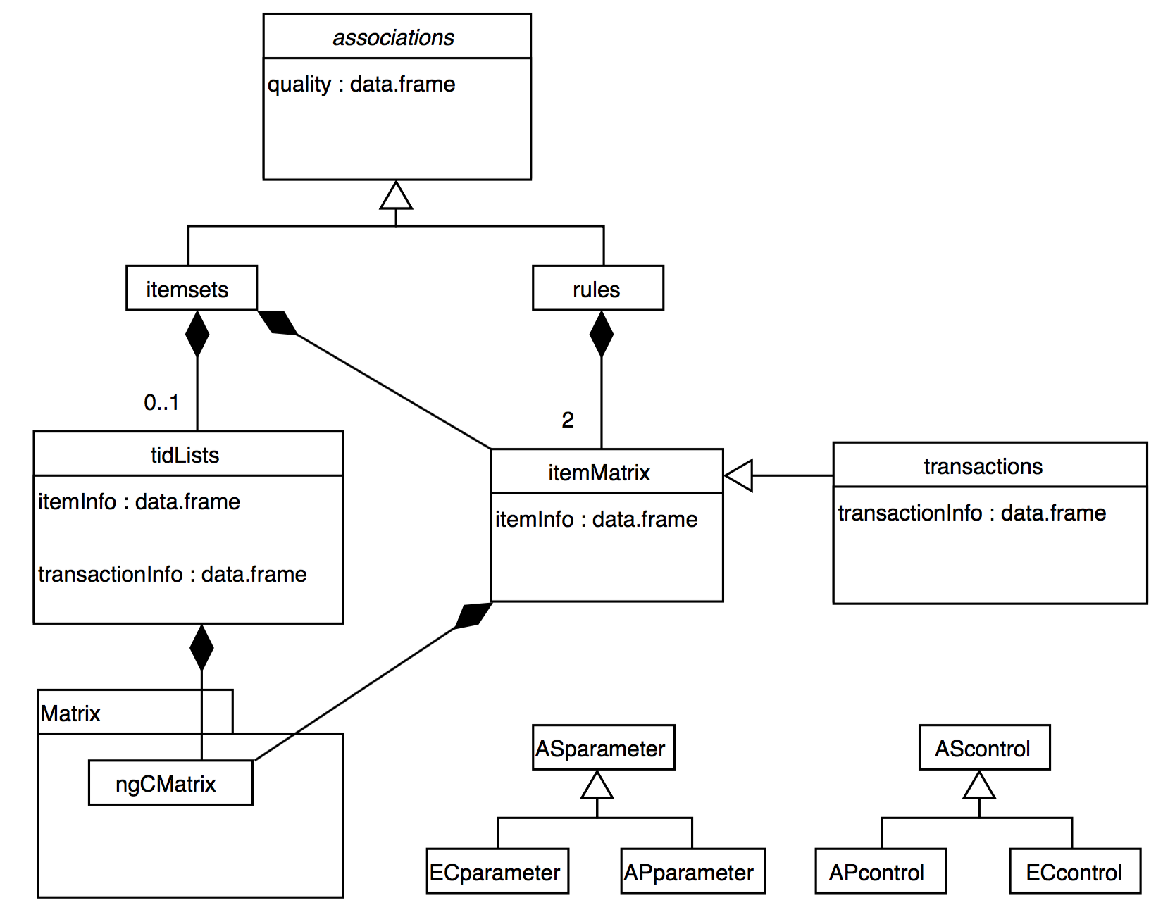
arules中的S4类的(数据)结构实现如下
关联规则示例
下面以arules包中的Groceries数据集为例子,介绍arules包的使用方法。Groceries 数据集是一个记录某个杂货店一个月真实交易记录的数据集
transactions
代码
library (arules)data ("Groceries" )summary (Groceries)
transactions as itemMatrix in sparse format with
 9835 rows (elements/itemsets/transactions) and
 169 columns (items) and a density of 0.02609146

most frequent items:
      whole milk other vegetables       rolls/buns             soda
            2513             1903             1809             1715
          yogurt          (Other)
            1372            34055

element (itemset/transaction) length distribution:
sizes
   1    2    3    4    5    6    7    8    9   10   11   12   13   14   15   16
2159 1643 1299 1005  855  645  545  438  350  246  182  117   78   77   55   46
  17   18   19   20   21   22   23   24   26   27   28   29   32
  29   14   14    9   11    4    6    1    1    1    1    3    1

   Min. 1st Qu.  Median    Mean 3rd Qu.    Max.
  1.000   2.000   3.000   4.409   6.000  32.000

includes extended item information - examples:
       labels  level2           level1
1 frankfurter sausage meat and sausage
2     sausage sausage meat and sausage
3  liver loaf sausage meat and sausage
通过summary展示transactions的概述,从summary返回的结果中可以看出:
Groceries是一个以稀疏矩阵存储的 项集矩阵(itemMatrix),总共有9835行(事务),169列(项),非零元素的比例(density)为0.02609146
Groceries中项集/事务的长度分布:包含1个项的有2159个事务,包含2个项的有1643个事务
Groceries中的事务数据中包含了 额外的 level 信息
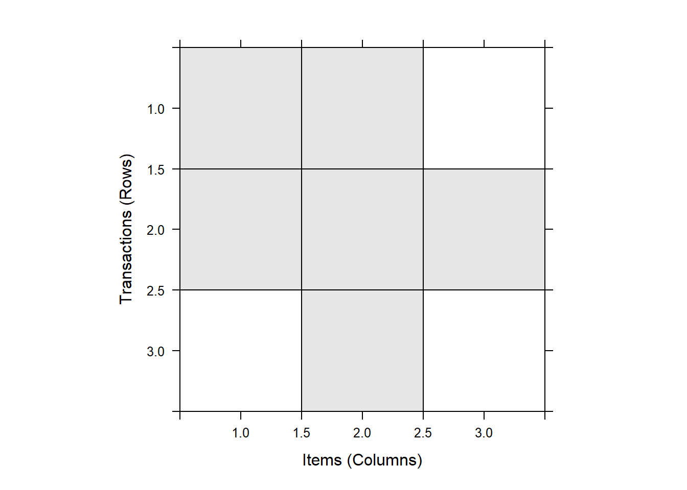
Transactions 是一种用于存储事务数据的数据结构。它是 itemMatrix 类的直接扩展,用于表示二进制的关联矩阵。每一行代表一个事务,每一列代表一个项。如果某个项在某个事务中出现,对应的矩阵元素为1;否则为0。
1.通过as可以将transactions的稀疏矩阵转为矩阵或者数据框等类型,别的类型数据也能通过as(,"transactions")转为事务数据
代码
as (Groceries[1 : 5 , 1 : 5 ], "matrix" )
     frankfurter sausage liver loaf   ham  meat
[1,]       FALSE   FALSE      FALSE FALSE FALSE
[2,]       FALSE   FALSE      FALSE FALSE FALSE
[3,]       FALSE   FALSE      FALSE FALSE FALSE
[4,]       FALSE   FALSE      FALSE FALSE FALSE
[5,]       FALSE   FALSE      FALSE FALSE FALSE
代码
as (head (Groceries), "data.frame" )
{citrus fruit,semi-finished bread,margarine,ready soups}
{tropical fruit,yogurt,coffee}
{whole milk}
{pip fruit,yogurt,cream cheese ,meat spreads}
{other vegetables,whole milk,condensed milk,long life bakery product}
{whole milk,butter,yogurt,rice,abrasive cleaner}
代码
as (head (Groceries), "list" )
[[1]]
[1] "citrus fruit"        "semi-finished bread" "margarine"
[4] "ready soups"

[[2]]
[1] "tropical fruit" "yogurt"         "coffee"

[[3]]
[1] "whole milk"

[[4]]
[1] "pip fruit"     "yogurt"        "cream cheese " "meat spreads"

[[5]]
[1] "other vegetables"         "whole milk"
[3] "condensed milk"           "long life bakery product"

[[6]]
[1] "whole milk"       "butter"           "yogurt"           "rice"
[5] "abrasive cleaner"
代码
as (head (Groceries), "tidLists" ) # 按水平布局的事务数据转换为垂直布局的事务ID列表
tidLists in sparse format with
 169 items/itemsets (rows) and
 6 transactions (columns)
2.将数据框转为Transactions
2.1 将数据框拆分后转换
代码
# 示例数据框 <- data.frame (TID = c (1 , 1 , 2 , 2 , 2 , 3 ),Item = c ("a" , "b" , "a" , "b" , "c" , "b" ),User = c ("UserA" , "UserA" , "UserB" , "UserC" , "UserC" , "UserC" ),Time = c ("2023-04-01 10:00:00" , "2023-04-01 10:00:00" , "2023-04-01 11:00:00" , "2023-04-01 11:00:00" , "2023-04-01 11:00:00" , "2023-04-01 12:40:00" )# 将数据框拆分并转换为 transactions 对象 <- as (split (df$ Item, df$ TID), "transactions" )summary (trans)
transactions as itemMatrix in sparse format with
 3 rows (elements/itemsets/transactions) and
 3 columns (items) and a density of 0.6666667

most frequent items:
      b       a       c (Other)
      3       2       1       0

element (itemset/transaction) length distribution:
sizes
1 2 3
1 1 1

   Min. 1st Qu.  Median    Mean 3rd Qu.    Max.
    1.0     1.5     2.0     2.0     2.5     3.0

includes extended item information - examples:
  labels
1      a
2      b
3      c

includes extended transaction information - examples:
  transactionID
1             1
2             2
3             3
2.2 将连续数据离散后转换
代码
<- discretizeDF (iris,methods = list (Petal.Length = list (method = "frequency" , breaks = 3 ,labels = c ("short" , "medium" , "long" )Petal.Width = list (method = "frequency" , breaks = 2 ,labels = c ("narrow" , "wide" )default = list (method = "none" )<- transactions (irisDisc[, c ("Petal.Length" , "Petal.Width" , "Species" )])inspect (head (iris_trans))
    items                 transactionID
[1] {Petal.Length=short,
     Petal.Width=narrow,
     Species=setosa}                  1
[2] {Petal.Length=short,
     Petal.Width=narrow,
     Species=setosa}                  2
[3] {Petal.Length=short,
     Petal.Width=narrow,
     Species=setosa}                  3
[4] {Petal.Length=short,
     Petal.Width=narrow,
     Species=setosa}                  4
[5] {Petal.Length=short,
     Petal.Width=narrow,
     Species=setosa}                  5
[6] {Petal.Length=short,
     Petal.Width=narrow,
     Species=setosa}                  6
3.修改项标签
代码
itemLabels (trans) <- c ("apple" , "banana" , "meat" )itemInfo (trans)$ Type <- c ("fruit" , "fruit" , "sausage" )summary (trans)
transactions as itemMatrix in sparse format with
 3 rows (elements/itemsets/transactions) and
 3 columns (items) and a density of 0.6666667

most frequent items:
 banana   apple    meat (Other)
      3       2       1       0

element (itemset/transaction) length distribution:
sizes
1 2 3
1 1 1

   Min. 1st Qu.  Median    Mean 3rd Qu.    Max.
    1.0     1.5     2.0     2.0     2.5     3.0

includes extended item information - examples:
  labels    Type
1  apple   fruit
2 banana   fruit
3   meat sausage

includes extended transaction information - examples:
  transactionID
1             1
2             2
3             3
4.添加额外的交易信息:设置交易用户与交易时间
代码
# 设置交易用户和交易时间 transactionInfo (trans)$ User <- unique (df$ User)transactionInfo (trans)$ Time <- unique (as.POSIXct (df$ Time, format = "%Y-%m-%d %H:%M:%S" ))summary (trans)
transactions as itemMatrix in sparse format with
 3 rows (elements/itemsets/transactions) and
 3 columns (items) and a density of 0.6666667

most frequent items:
 banana   apple    meat (Other)
      3       2       1       0

element (itemset/transaction) length distribution:
sizes
1 2 3
1 1 1

   Min. 1st Qu.  Median    Mean 3rd Qu.    Max.
    1.0     1.5     2.0     2.0     2.5     3.0

includes extended item information - examples:
  labels    Type
1  apple   fruit
2 banana   fruit
3   meat sausage

includes extended transaction information - examples:
  transactionID  User                Time
1             1 UserA 2023-04-01 10:00:00
2             2 UserB 2023-04-01 11:00:00
3             3 UserC 2023-04-01 12:40:00
代码
    items                 transactionID User  Time
[1] {apple, banana}       1             UserA 2023-04-01 10:00:00
[2] {apple, banana, meat} 2             UserB 2023-04-01 11:00:00
[3] {banana}              3             UserC 2023-04-01 12:40:00
5.itemMatrix的常用操作
代码
代码
# 获取事务数据集的项集数量(行数目) length (trans)
代码
# 检查是否有重复的事务 duplicated (trans)
代码
# 获取事务数据集中的唯一项 unique (trans)
transactions in sparse format with
 3 transactions (rows) and
 3 items (columns)
代码
代码
# 计算每个项在事务数据集中的频率 itemFrequency (trans)
    apple    banana      meat
0.6666667 1.0000000 0.3333333
代码
查看事务分布
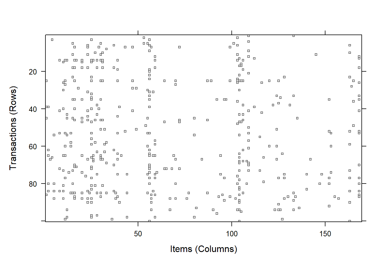
通过image可以查看数据分布情况,数据量较大时,可以使用sample进行抽样
代码
<- sample (Groceries, 100 )image (Groceries100, replace = FALSE )
代码
# image(Groceries[1:100,itemInfo(Groceries)$level1=='drinks'])
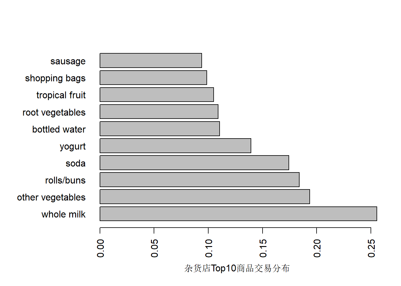
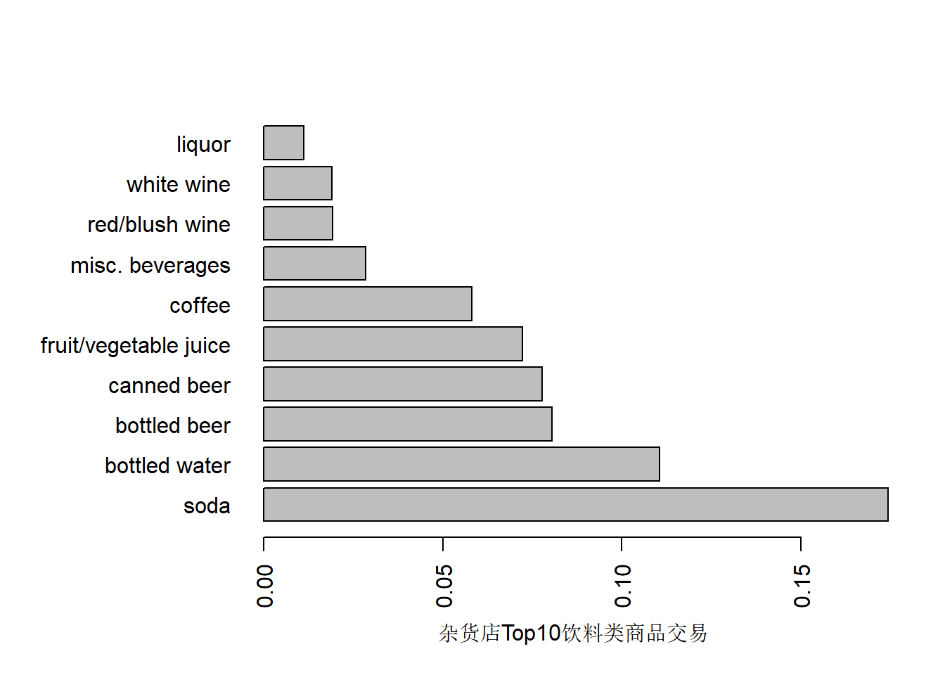
itemFrequencyPlot可以查看项集分布情况
代码
itemFrequencyPlot (Groceries,topN = 10 , xlab = "杂货店Top10商品交易分布" , horiz = T,names = TRUE itemFrequencyPlot (Groceries[, itemInfo (Groceries)$ level1 == "drinks" ],topN = 10 ,names = TRUE , horiz = T, xlab = "杂货店Top10饮料类商品交易"
通过size查看较长的事务,确认是否较长的事务为异常数据
代码
inspect (Groceries[size (Groceries) > 30 , ])
    items
[1] {frankfurter,
     sausage,
     liver loaf,
     ham,
     chicken,
     beef,
     citrus fruit,
     tropical fruit,
     root vegetables,
     other vegetables,
     whole milk,
     butter,
     curd,
     yogurt,
     whipped/sour cream,
     beverages,
     soft cheese,
     hard cheese,
     cream cheese ,
     mayonnaise,
     domestic eggs,
     rolls/buns,
     roll products ,
     flour,
     pasta,
     margarine,
     specialty fat,
     sugar,
     soups,
     skin care,
     hygiene articles,
     candles}
关联规则构建
代码
<- apriori (Groceries,parameter = list (support = 0.001 , confidence = 0.8 )
Apriori

Parameter specification:
 confidence minval smax arem  aval originalSupport maxtime support minlen
        0.8    0.1    1 none FALSE            TRUE       5   0.001      1
 maxlen target  ext
     10  rules TRUE

Algorithmic control:
 filter tree heap memopt load sort verbose
    0.1 TRUE TRUE  FALSE TRUE    2    TRUE

Absolute minimum support count: 9

set item appearances ...[0 item(s)] done [0.00s].
set transactions ...[169 item(s), 9835 transaction(s)] done [0.00s].
sorting and recoding items ... [157 item(s)] done [0.00s].
creating transaction tree ... done [0.00s].
checking subsets of size 1 2 3 4 5 6 done [0.01s].
writing ... [410 rule(s)] done [0.00s].
creating S4 object  ... done [0.00s].
代码
inspect (head (sort (rules, by = "lift" )))
    lhs                        rhs                   support confidence    coverage      lift count
[1] {liquor,
     red/blush wine}        => {bottled beer}    0.001931876  0.9047619 0.002135231 11.235269    19
[2] {citrus fruit,
     other vegetables,
     soda,
     fruit/vegetable juice} => {root vegetables} 0.001016777  0.9090909 0.001118454  8.340400    10
[3] {tropical fruit,
     other vegetables,
     whole milk,
     yogurt,
     oil}                   => {root vegetables} 0.001016777  0.9090909 0.001118454  8.340400    10
[4] {citrus fruit,
     grapes,
     fruit/vegetable juice} => {tropical fruit}  0.001118454  0.8461538 0.001321810  8.063879    11
[5] {other vegetables,
     whole milk,
     yogurt,
     rice}                  => {root vegetables} 0.001321810  0.8666667 0.001525165  7.951182    13
[6] {tropical fruit,
     other vegetables,
     whole milk,
     oil}                   => {root vegetables} 0.001321810  0.8666667 0.001525165  7.951182    13
按提升度 从高到低排序,从第一行数据,可以看到:
lhs (左手边项) :包含两种酒类:烈酒 和红/粉红葡萄酒 。
rhs (右手边项) :这是另一种酒类,即瓶装啤酒 。
支持度 (support) :支持度是指同时购买左手边项和右手边项的比例。在这里,支持度为约0.19%,表示这lhs和rhs的同时购买发生的频率很低。
置信度 (confidence) :置信度是指在购买左手边项的情况下,同时购买右手边项的概率。在这里,置信度为约90.48%,表示购买烈酒和红/粉红葡萄酒的顾客中,有90.48% 也会购买瓶装啤酒。
覆盖率 (coverage) :覆盖率是指购买左手边项。在这里,覆盖率为约0.21%,表示购买烈酒和红/粉红葡萄酒的顾客占总体购买人群的比例。
提升度 (lift) :提升度是指同时购买左手边项和右手边项的概率与各自独立购买的概率之比。在这里,提升度为约11.24,表示购买烈酒和红/粉红葡萄酒时,同时购买瓶装啤酒的概率比整体瓶装啤酒购买时高出11.24倍。
提取目标规则
通过apriori可以找到大量的关联规则,但是一般来说,我们只会关心其中一部分,通过subset可以抽取指定的关联规则
代码
<- subset (rules, subset = rhs %pin% "root vegetables" & lift > 3 )inspect (rulesRootvegetables)
    lhs                        rhs                   support confidence    coverage     lift count
[1] {other vegetables,
     whole milk,
     yogurt,
     rice}                  => {root vegetables} 0.001321810  0.8666667 0.001525165 7.951182    13
[2] {tropical fruit,
     other vegetables,
     whole milk,
     oil}                   => {root vegetables} 0.001321810  0.8666667 0.001525165 7.951182    13
[3] {beef,
     citrus fruit,
     tropical fruit,
     other vegetables}      => {root vegetables} 0.001016777  0.8333333 0.001220132 7.645367    10
[4] {citrus fruit,
     other vegetables,
     soda,
     fruit/vegetable juice} => {root vegetables} 0.001016777  0.9090909 0.001118454 8.340400    10
[5] {tropical fruit,
     other vegetables,
     whole milk,
     yogurt,
     oil}                   => {root vegetables} 0.001016777  0.9090909 0.001118454 8.340400    10
导出关联规则
通过write及write.PMML可以将提取到的关联规则写入文件
代码
write (rules, file = "data.csv" , sep = "," , col.names = NA )write.PMML (rules, file = "data.xml" )
事务数据抽样
在一些情况下,我们可能面临大量的事务数据,我们的计算机可能无法快速的完成关联规则的计算,这时候我们可以采取抽样。Zaki等认为对于持度为τ=supp(X)的项集X,在给定置信水平1−c下可接受的支持度相对误差为ϵ时,抽样数据集所需的大小n可以计算
\[n=\frac{-2ln(c)}{τϵ^2}\]
代码
<- 0.05 <- 0.1 <- 0.3 <- - 2 * log (c) / (supp * epsilon^ 2 )
代码
<- sample (Groceries, n)
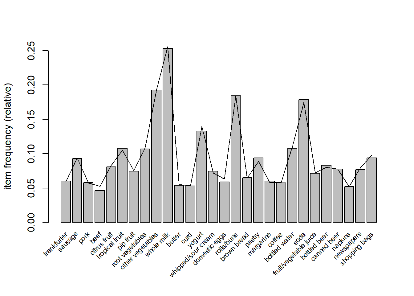
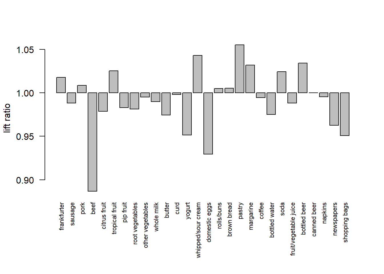
itemFrequencyPlot的 population参数可以查看样本与总体的分布差异,样本集的项频率显示为长条,原始数据库的项频率表示为线。另外,样本可以通过提升率(lift ratio)将样本集与总体进行比较:每个项i 的提升率(lift ration)定义为\(\frac{P(i|sample)}{P(i|population)}\) ,其中概率通过项的频率估计。
代码
itemFrequencyPlot (GroceriesSample,population = Groceries, support = 0.05 ,cex.names = 0.7 itemFrequencyPlot (GroceriesSample,population = Groceries, support = 0.05 ,cex.names = 0.7 , lift = TRUE
时间对比
代码
<- system.time (itemsets <- eclat (Groceries,parameter = list (support = supp), control = list (verbose = FALSE )
   user  system elapsed
   0.01    0.00    0.00
代码
<- system.time (itemsetsSample <- eclat (GroceriesSample,parameter = list (support = supp), control = list (verbose = FALSE )
   user  system elapsed
      0       0       0
Apriori 算法 :
适用于大型数据集。
扫描原始(真实)数据集。
通过计算候选项集的支持度来生成频繁项集。
相对较慢,因为需要多次扫描数据集。
使用水平搜索方式。
Eclat 算法 :
更适合中小型数据集。
扫描当前生成的数据集。
使用深度优先搜索方式。
通常比 Apriori 算法更快。
使用的内存较少,因为采用了深度优先搜索方法。
结果对比
可以看出样本生成的规则覆盖了总体生成的所有规则
代码
<- match (itemsets, itemsetsSample, nomatch = 0 )sum (matchrule > 0 ) / length (itemsets)
关联聚类
代码
library (plotly)library (dendextend)<- Groceries[, itemFrequency (Groceries) > 0.05 ]<- dissimilarity (s, which = "items" )# plot(hclust(d_jaccard, method = "ward.D2"), main = "Dendrogram for items") hclust (d_jaccard, method = "ward.D2" ) %>% as.dendrogram () %>% plot_dendro (xmin = - 0.3 , width = 800 , height = 500 )
顺序项集挖掘
arulesSequence 包是arules的一个扩展功能包,它专门用于序列分析,可以发现项目之间的时间或顺序依赖性。
定义说明
事件流:记录用户进行操作的按照时间排序的有序事件记录
子事件流:任何一个长度为n的事件流都包含着 \(2^n-1\) 个子事件流,
例如事件流:<{a},{b},{c},{d}>包含的子事件流为:
1:<{a}> 2:<{b}> 3:<{c}> 4:<{d}> 5:<{a},{b}> 6:<{a},{c}> 7:<{a},{d}> 8:<{b},{c}> 9:<{b},{d}> 10:<{c},{d}> 11:<{a},{b},{c}> 12:<{a},{b},{d}> 13:<{a},{c},{d}> 14:<{b},{c},{d}> 15:<{a},{b},{c},{d}>
数据准备
代码
set.seed (123 )# 生成示例数据 library (timetk)library (dplyr)library (stringr)library (arulesSequences)<- data.frame (sequenceID = sample (1 : 5 , 20 , replace = T),Item = sample (c ("a" , "b" , "c" , "d" , "e" ), 20 , replace = T),Time = sample (tk_make_timeseries ("2024-01-01 01:01:00" , "2024-01-01 01:03:00" , by = "1 min" ), 20 , replace = T)%>% arrange (sequenceID, Time, Item) %>% unique () %>% group_by (sequenceID) %>% mutate (eventID = dense_rank (Time)) %>% ungroup () %>% group_by (sequenceID, eventID) %>% summarise (SIZE = n (), items = str_c (Item, collapse = ";" ))
1
1
1
e
1
2
3
c;d;e
2
1
2
b;d
2
2
1
b
2
3
1
c
3
1
2
a;b
3
2
2
a;e
3
3
1
a
4
1
1
e
4
2
1
d
5
1
2
a;c
5
2
1
c
代码
write.table (df, "example.txt" , sep = ";" , row.names = FALSE , col.names = FALSE , quote = FALSE )<- read_baskets ("example.txt" , sep = ";" , info = c ("sequenceID" , "eventID" , "SIZE" ))# 查看序列数据 inspect (trans)
     items     sequenceID eventID SIZE
[1]  {e}       1          1       1
[2]  {c, d, e} 1          2       3
[3]  {b, d}    2          1       2
[4]  {b}       2          2       1
[5]  {c}       2          3       1
[6]  {a, b}    3          1       2
[7]  {a, e}    3          2       2
[8]  {a}       3          3       1
[9]  {e}       4          1       1
[10] {d}       4          2       1
[11] {a, c}    5          1       2
[12] {c}       5          2       1
支持度计算
通过cspade计算出各序列的支持度,parameter参数可以限制序列的长度,支持度等
代码
<- cspade (trans,parameter = list (support = 0 ,maxsize = 1 , maxlen = 2 ,maxgap = 5 # 限制时间的差异最大值(eventID) control = list (verbose = TRUE )
parameter specification:
support : 0
maxsize : 1
maxlen  : 2
maxgap  : 5

algorithmic control:
bfstype  : FALSE
verbose  :  TRUE
summary  : FALSE
tidLists : FALSE

preprocessing ... 1 partition(s), 0 MB [0.16s]
mining transactions ... 0 MB [0.09s]
reading sequences ... [0.02s]

total elapsed time: 0.27s
代码
    items support
  1 <{a}>     0.4
  2 <{b}>     0.4
  3 <{c}>     0.6
  4 <{d}>     0.6
  5 <{e}>     0.6
  6 <{a},
     {e}>     0.2
  7 <{b},
     {e}>     0.2
  8 <{e},
     {e}>     0.2
  9 <{e},
     {d}>     0.4
 10 <{a},
     {c}>     0.2
 11 <{b},
     {c}>     0.2
 12 <{c},
     {c}>     0.2
 13 <{d},
     {c}>     0.2
 14 <{e},
     {c}>     0.2
 15 <{b},
     {b}>     0.2
 16 <{d},
     {b}>     0.2
 17 <{a},
     {a}>     0.2
 18 <{b},
     {a}>     0.2
 19 <{e},
     {a}>     0.2
序列关联规则
更进一步,通过ruleInduction计算序列关联规则
代码
<- ruleInduction (s0,confidence = .5 ,control = list (verbose = TRUE )inspect (r0)
   lhs      rhs   support confidence      lift
 1 <{a}> => <{e}>     0.2  0.5000000 0.8333333
 2 <{b}> => <{e}>     0.2  0.5000000 0.8333333
 3 <{e}> => <{d}>     0.4  0.6666667 1.1111111
 4 <{a}> => <{c}>     0.2  0.5000000 0.8333333
 5 <{b}> => <{c}>     0.2  0.5000000 0.8333333
 6 <{b}> => <{b}>     0.2  0.5000000 1.2500000
 7 <{a}> => <{a}>     0.2  0.5000000 1.2500000
 8 <{b}> => <{a}>     0.2  0.5000000 1.2500000
解读以上首行数据<{a}> => <{e}>
support=0.2:先{a}后{e}的数据有1条,占总的(5条序列)的20%
confidence=0.5:包含{a}的数据序列有2条,{a}后{e}的数据有1条,占包含{a}的序列的50%
lift=0.8333333 :相较于整体的提升度,在整体中包含{e}的序列有3条,占0.6(即覆盖率),lift = confidence / coverage = 0.5/0.6
序列分类
可以通过在trans中添加classID,来区分不同的类别人群的序列,比如classID为2的代表下单人群,classID为1的代表未转化人群
代码
transactionInfo (trans)$ classID <- as.integer (transactionInfo (trans)$ sequenceID) %% 2 + 1 Linspect (trans)
     items     sequenceID eventID SIZE classID
[1]  {e}       1          1       1    2
[2]  {c, d, e} 1          2       3    2
[3]  {b, d}    2          1       2    1
[4]  {b}       2          2       1    1
[5]  {c}       2          3       1    1
[6]  {a, b}    3          1       2    2
[7]  {a, e}    3          2       2    2
[8]  {a}       3          3       1    2
[9]  {e}       4          1       1    1
[10] {d}       4          2       1    1
[11] {a, c}    5          1       2    2
[12] {c}       5          2       1    2
解读以下首行结果数据:整体中有40%的序列中有{a},未转化人群中没有人有{a},转化人群中有66.6%有{a},可以猜测{a}对下单转化有较大的影响。
代码
<- cspade (trans,parameter = list (support = 0 ,maxsize = 1 , maxlen = 2 control = list (verbose = F)inspect (s1)
    items support   1         2
  1 <{a}>     0.4 0.0 0.6666667
  2 <{b}>     0.4 0.5 0.3333333
  3 <{c}>     0.6 0.5 0.6666667
  4 <{d}>     0.6 1.0 0.3333333
  5 <{e}>     0.6 0.5 0.6666667
  6 <{a},
     {e}>     0.2 0.0 0.3333333
  7 <{b},
     {e}>     0.2 0.0 0.3333333
  8 <{e},
     {e}>     0.2 0.0 0.3333333
  9 <{e},
     {d}>     0.4 0.5 0.3333333
 10 <{a},
     {c}>     0.2 0.0 0.3333333
 11 <{b},
     {c}>     0.2 0.5 0.0000000
 12 <{c},
     {c}>     0.2 0.0 0.3333333
 13 <{d},
     {c}>     0.2 0.5 0.0000000
 14 <{e},
     {c}>     0.2 0.0 0.3333333
 15 <{b},
     {b}>     0.2 0.5 0.0000000
 16 <{d},
     {b}>     0.2 0.5 0.0000000
 17 <{a},
     {a}>     0.2 0.0 0.3333333
 18 <{b},
     {a}>     0.2 0.0 0.3333333
 19 <{e},
     {a}>     0.2 0.0 0.3333333
Python
Python的mlxtend也能用于关联规则
代码
import pandas as pdfrom mlxtend.preprocessing import TransactionEncoderfrom mlxtend.frequent_patterns import apriori, fpmax, fpgrowth= [['Milk' , 'Onion' , 'Nutmeg' , 'Kidney Beans' , 'Eggs' , 'Yogurt' ],'Dill' , 'Onion' , 'Nutmeg' , 'Kidney Beans' , 'Eggs' , 'Yogurt' ],'Milk' , 'Apple' , 'Kidney Beans' , 'Eggs' ],'Milk' , 'Unicorn' , 'Corn' , 'Kidney Beans' , 'Yogurt' ],'Corn' , 'Onion' , 'Onion' , 'Kidney Beans' , 'Ice cream' , 'Eggs' ]]= TransactionEncoder()= te.fit(dataset).transform(dataset)= pd.DataFrame(te_ary, columns= te.columns_)= fpgrowth(df, min_support= 0.6 , use_colnames= True )### alternatively: #frequent_itemsets = apriori(df, min_support=0.6, use_colnames=True) #frequent_itemsets = fpmax(df, min_support=0.6, use_colnames=True)
    support                     itemsets
0       1.0               (Kidney Beans)
1       0.8                       (Eggs)
2       0.6                     (Yogurt)
3       0.6                       (Milk)
4       0.6                      (Onion)
5       0.8         (Kidney Beans, Eggs)
6       0.6       (Kidney Beans, Yogurt)
7       0.6         (Milk, Kidney Beans)
8       0.6                (Eggs, Onion)
9       0.6        (Kidney Beans, Onion)
10      0.6  (Kidney Beans, Eggs, Onion)
代码
from mlxtend.frequent_patterns import association_rules= "confidence" , min_threshold= 0.7 )
              antecedents            consequents  ...  certainty  kulczynski
0          (Kidney Beans)                 (Eggs)  ...      0.000       0.900
1                  (Eggs)         (Kidney Beans)  ...      0.000       0.900
2                (Yogurt)         (Kidney Beans)  ...      0.000       0.800
3                  (Milk)         (Kidney Beans)  ...      0.000       0.800
4                  (Eggs)                (Onion)  ...      0.375       0.875
5                 (Onion)                 (Eggs)  ...      1.000       0.875
6                 (Onion)         (Kidney Beans)  ...      0.000       0.800
7    (Kidney Beans, Eggs)                (Onion)  ...      0.375       0.875
8   (Kidney Beans, Onion)                 (Eggs)  ...      1.000       0.875
9           (Eggs, Onion)         (Kidney Beans)  ...      0.000       0.800
10                 (Eggs)  (Kidney Beans, Onion)  ...      0.375       0.875
11                (Onion)   (Kidney Beans, Eggs)  ...      1.000       0.875

[12 rows x 14 columns]