模型介绍
评分卡模型是一种常用于信用风险评估的模型,通常用于预测个体的违约概率或信用风险。
评分卡模型基于统计学和机器学习技术,通过将各种变量(如个人信息、财务信息等)转化为分数来评估个体的信用风险水平。
评分卡模型的基本原理是根据历史数据和违约情况建立一个预测模型,该模型可以根据个体的特征给出一个信用评分,该评分反映了个体发生违约的可能性。
数据集
GermanCredit数据集是一个经典的信用风险评估数据集,通常用于机器学习和数据分析的教学和实践。该数据集包含了德国银行客户的个人信息和信用情况,以及他们是否违约的标签信息。下面是该数据集的一些基本信息:
数据集包含1000个样本,每个样本有20个特征变量和1个目标变量。
特征变量包括客户的个人信息(如性别、年龄、婚姻状况)、财务信息(如贷款金额、贷款期限、存款金额)、工作信息等。
代码
library (scorecard)data ("germancredit" ):: skim (germancredit)
Data summary
Name
germancredit
Number of rows
1000
Number of columns
21
_______________________
Column type frequency:
character
1
factor
13
numeric
7
________________________
Group variables
None
Variable type: character
Variable type: factor
status.of.existing.checking.account
0
1
FALSE
4
no : 394, …: 274, 0 <: 269, …: 63
credit.history
0
1
FALSE
5
exi: 530, cri: 293, del: 88, all: 49
savings.account.and.bonds
0
1
FALSE
5
…: 603, unk: 183, 100: 103, 500: 63
present.employment.since
0
1
FALSE
5
1 <: 339, …: 253, 4 <: 174, …: 172
personal.status.and.sex
0
1
FALSE
4
mal: 548, fem: 310, mal: 92, mal: 50
other.debtors.or.guarantors
0
1
FALSE
3
non: 907, gua: 52, co-: 41
property
0
1
FALSE
4
car: 332, rea: 282, bui: 232, unk: 154
other.installment.plans
0
1
FALSE
3
non: 814, ban: 139, sto: 47
housing
0
1
FALSE
3
own: 713, ren: 179, for: 108
job
0
1
FALSE
4
ski: 630, uns: 200, man: 148, une: 22
telephone
0
1
FALSE
2
non: 596, yes: 404
foreign.worker
0
1
FALSE
2
yes: 963, no: 37
creditability
0
1
FALSE
2
goo: 700, bad: 300
Variable type: numeric
duration.in.month
0
1
20.90
12.06
4
12.0
18.0
24.00
72
▇▇▂▁▁
credit.amount
0
1
3271.26
2822.74
250
1365.5
2319.5
3972.25
18424
▇▂▁▁▁
installment.rate.in.percentage.of.disposable.income
0
1
2.97
1.12
1
2.0
3.0
4.00
4
▂▃▁▂▇
present.residence.since
0
1
2.85
1.10
1
2.0
3.0
4.00
4
▂▆▁▃▇
age.in.years
0
1
35.55
11.38
19
27.0
33.0
42.00
75
▇▆▃▁▁
number.of.existing.credits.at.this.bank
0
1
1.41
0.58
1
1.0
1.0
2.00
4
▇▅▁▁▁
number.of.people.being.liable.to.provide.maintenance.for
0
1
1.16
0.36
1
1.0
1.0
1.00
2
▇▁▁▁▂
数据清洗
代码
<- var_filter (germancredit, y = "creditability" , lims = list (missing_rate = 0.95 ,identical_rate = 0.95 , info_value = 0.02 var_rm = c ("installment.rate.in.percentage.of.disposable.income" ), var_kp = c ("duration.in.month" ,"credit.history" , "purpose" , "credit.amount" , "savings.account.and.bonds" , "job"
✔ 1 variables are removed via identical_rate
✔ 5 variables are removed via info_value
✔ Variable filtering on 1000 rows and 20 columns in 00:00:00
✔ 7 variables are removed in total
lims:是一个列表,包含了三个筛选条件:
missing_rate = 0.95:表示如果某个变量的缺失率超过95%,则将其删除。 i
dentical_rate = 0.95:表示如果某个变量的取值完全相同的比例超过95%,则将其删除。
info_value = 0.02:表示如果某个变量的信息价值(IV)低于0.02,说明该变量对目标变量的预测能力较弱,将其删除。
信息价值(Information Value,IV)是衡量一个特征变量对目标变量的预测能力的指标,通常用于评估变量在二分类问题中的重要性。信息价值的计算通常包括以下步骤:
计算每个特征变量的分箱(binning):将连续型变量离散化为若干个分箱,或者对离散型变量进行分组,以便后续计算IV。
对每个分箱计算如下指标:
正样本数量(Positive Count):该分箱中目标变量为正类别的样本数量。
负样本数量(Negative Count):该分箱中目标变量为负类别的样本数量。
正样本比例(Positive Rate):正样本数量占该分箱样本总数的比例。
负样本比例(Negative Rate):负样本数量占该分箱样本总数的比例。
计算每个分箱的证据权重(Weight of ,WOE):
WOE表示正样本比例与负样本比例的对数比值的自然对数。公式如下:
\[
WOE=ln(\frac{正样本比例} {负样本比例})
\]
计算IV值:
IV表示该分箱中正负样本比例差异对模型预测的影响程度。公式如下:
\[
IV = \sum_{i=1}^{n}(正样本比例_i - 负样本比例_i) \times WOE_i
\]
IV值的设计有以下几个原因:
对数比值的转换:IV值的计算基于对数比值(WOE),这种转换可以将正负样本比例的差异转化为线性关系,更好地反映了特征变量对目标变量的影响程度。
区分度和稳定性:IV值不仅考虑了特征变量不同分箱中正负样本比例的差异,还通过对数比值的转换增强了区分度和稳定性。这样可以更准确地评估特征变量的预测能力。
简单直观:IV值的计算简单直观,通过对正负样本比例的差异进行加权求和,可以直观地反映特征变量在不同分箱中的影响程度,便于理解和解释。
可比性:IV值的范围固定在0到正无穷,不受样本量和特征变量取值范围的影响,使得不同特征变量的IV值具有可比性,可以用于特征选择和模型评估。
通常情况下,IV值的范围如下:
通过计算信息价值,可以帮助选择对目标变量预测能力较强的特征变量,从而提高模型的准确性和泛化能力。
划分数据
代码
<- split_df (dt_f, y = "creditability" , ratios = c (0.6 , 0.4 ), seed = 30 )<- lapply (dt_list, function (x) x$ creditability)
计算IV
WOE是通过比较每个分箱内正负样本的比例来计算的,它表示了特征变量在不同分箱中对目标变量的影响程度。
WOE用于评估特征变量在不同分箱内的预测能力,可以帮助选择合适的分箱方案。
IV则用于衡量特征变量整体对目标变量的预测能力,可以帮助筛选对模型预测能力有贡献的特征变量。
代码
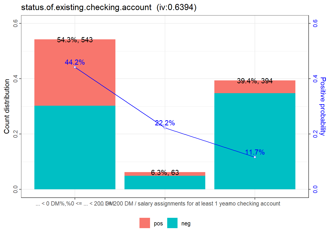
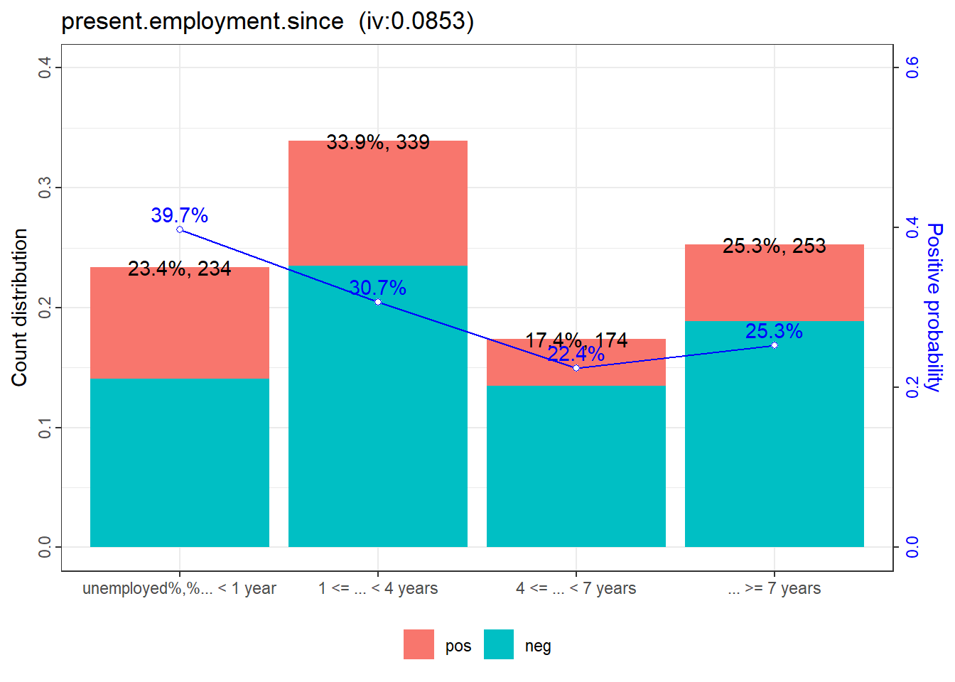
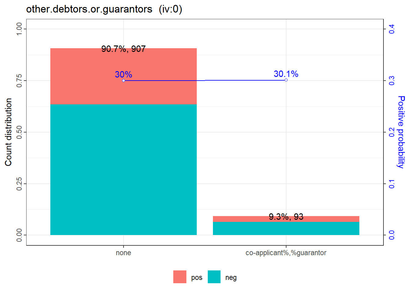
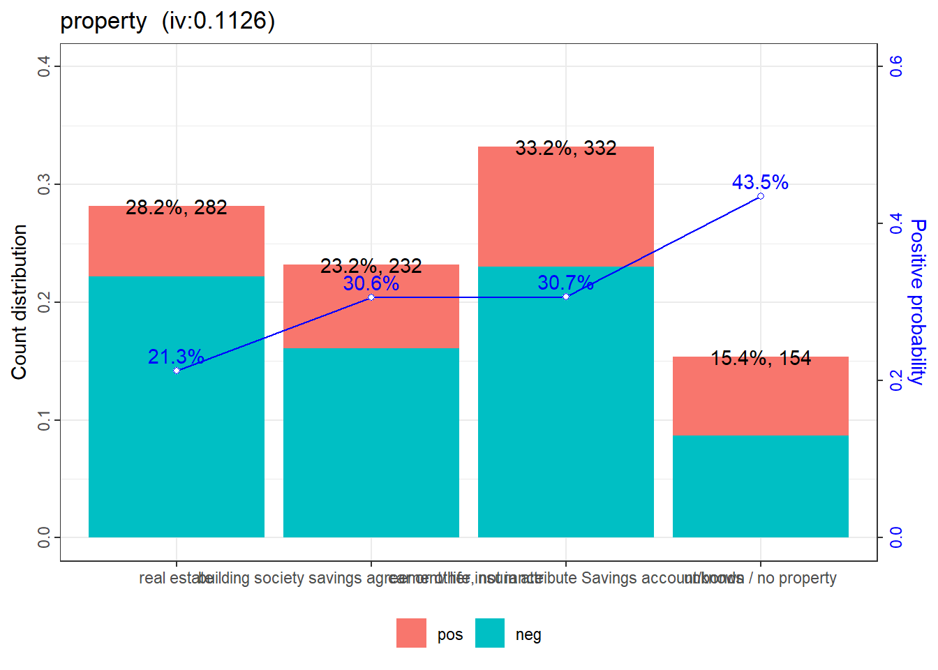
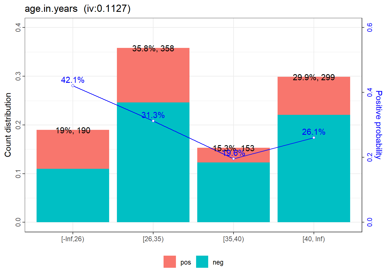
# bins <- woebin(dt_f, y = "creditability") ## 手动设置指定变量的划分,未手动设置的会自动计算划分分箱 <- list (age.in.years = c (26 , 35 , 40 ),other.debtors.or.guarantors = c ("none" , "co-applicant%,%guarantor" )<- woebin (dt_f, y = "creditability" , breaks_list = breaks_adj)<- woebin_plot (bins_adj)
✔ Binning on 1000 rows and 14 columns in 00:00:01
代码
for (p in woe_plot) {print (p)
代码
iv (dt_f, y = "creditability" )
variable info_value
<char> <num>
1: status.of.existing.checking.account 0.666011503
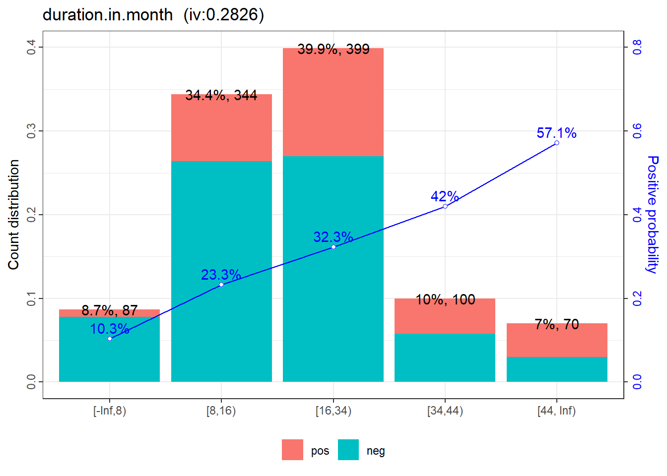
2: duration.in.month 0.334503490
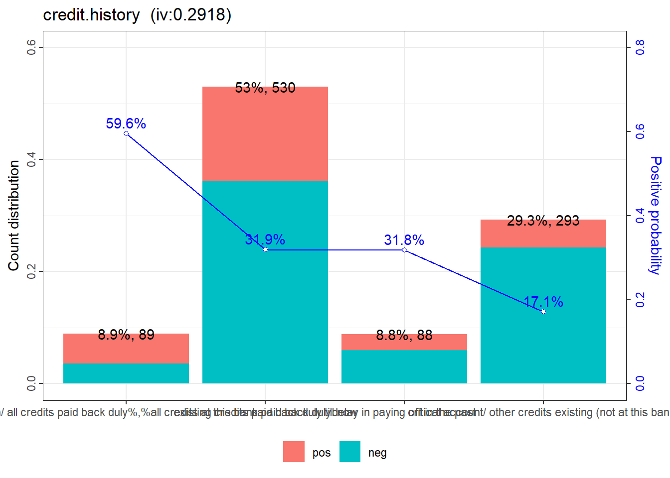
3: credit.history 0.293233547
4: age.in.years 0.259651423
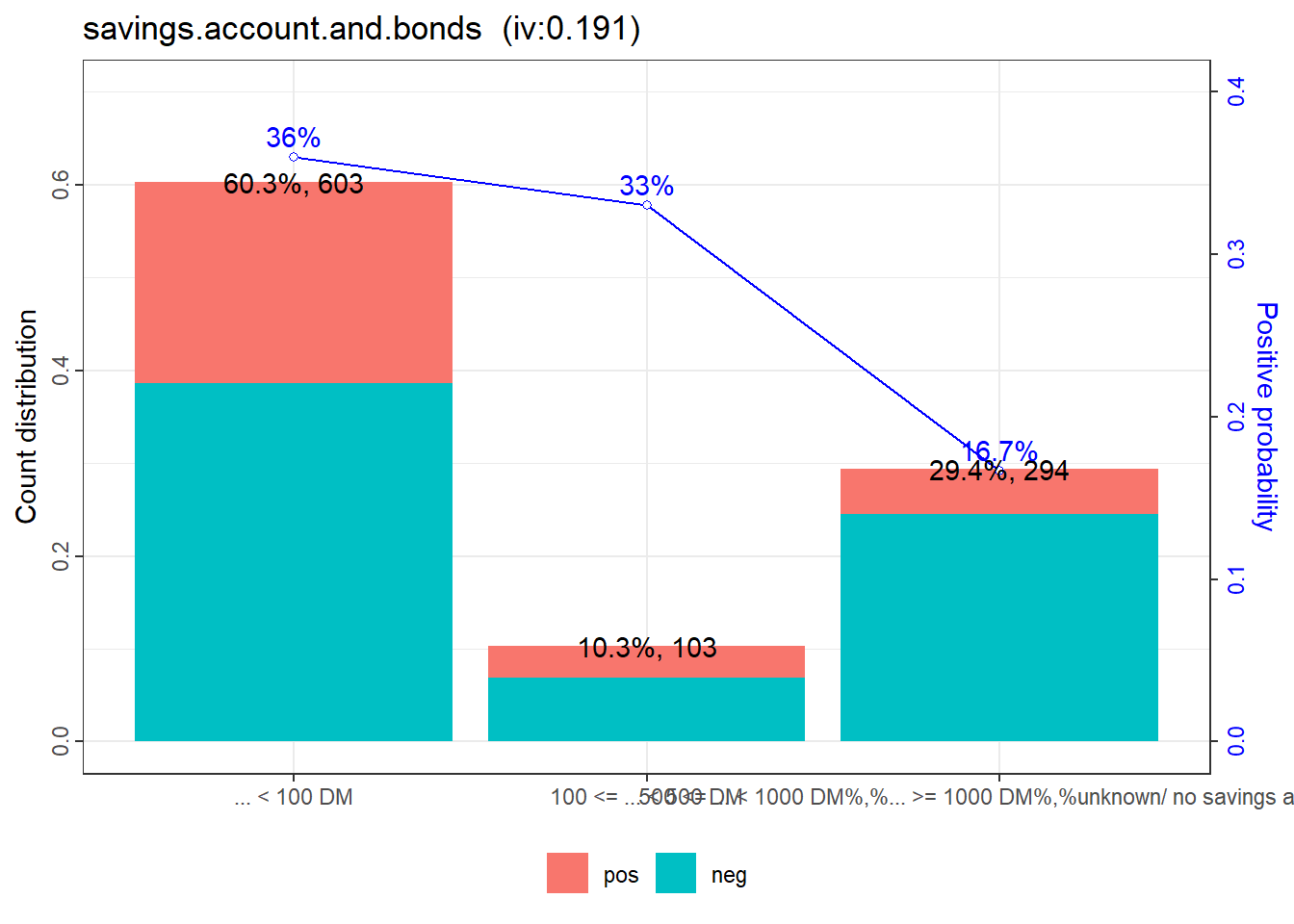
5: savings.account.and.bonds 0.196009557
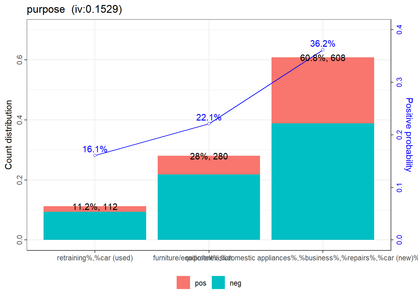
6: purpose 0.169195066
7: property 0.112638262
8: present.employment.since 0.086433631
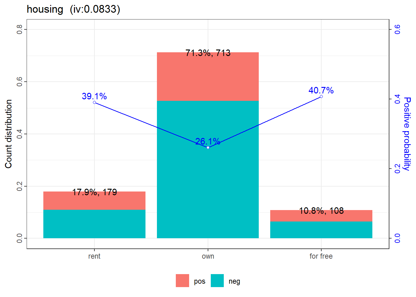
9: housing 0.083293434
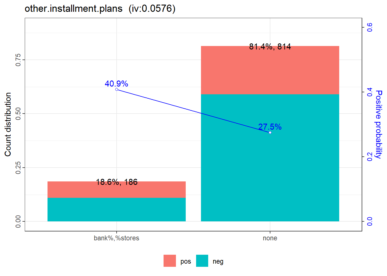
10: other.installment.plans 0.057614542
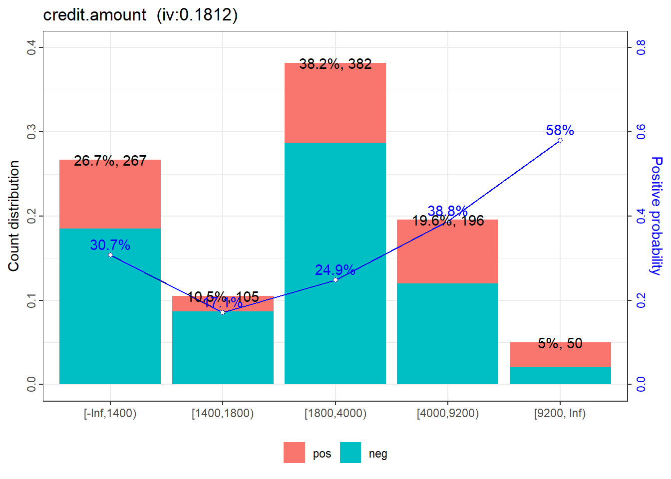
11: credit.amount 0.038957265
12: other.debtors.or.guarantors 0.032019322
13: job 0.008762766
根据IV值的排序,可以看出”status.of.existing.checking.account”对目标变量的预测能力最强,而”job”的预测能力最弱。
模型训练与评估
逻辑回归
代码
<- lapply (dt_list, function (x) woebin_ply (x, bins_adj))
✔ Woe transformating on 620 rows and 13 columns in 00:00:00
✔ Woe transformating on 380 rows and 13 columns in 00:00:00
代码
<- glm (creditability ~ ., family = binomial (), data = dt_woe_list$ train)vif (m1, merge_coef = TRUE )
                                   variable    Estimate Std. Error z value
                                     <char>       <num>      <num>   <num>
 1:                             (Intercept)  -0.9420468     0.1080 -8.7234
 2: status.of.existing.checking.account_woe   0.7395712     0.1379  5.3638
 3:            present.employment.since_woe   0.4501553     0.3530  1.2753
 4:         other.debtors.or.guarantors_woe -59.0105980    62.5310 -0.9437
 5:                            property_woe   0.3664055     0.3630  1.0093
 6:                        age.in.years_woe   0.9479652     0.3264  2.9043
 7:             other.installment.plans_woe   0.8051799     0.4284  1.8795
 8:                             housing_woe   0.6622283     0.3871  1.7109
 9:                   duration.in.month_woe   0.7951651     0.2315  3.4351
10:                      credit.history_woe   0.7665071     0.2012  3.8095
11:                             purpose_woe   0.8399740     0.2730  3.0773
12:                       credit.amount_woe   0.6183492     0.2793  2.2137
13:           savings.account.and.bonds_woe   0.7549808     0.2592  2.9125
14:                                 job_woe  -0.4809787     1.2026 -0.4000
    Pr(>|z|)     gvif
       <num>    <num>
 1:   0.0000       NA
 2:   0.0000 1.046089
 3:   0.2022 1.059807
 4:   0.3453 1.043887
 5:   0.3128 1.413885
 6:   0.0037 1.116636
 7:   0.0602 1.066091
 8:   0.0871 1.200516
 9:   0.0006 1.259093
10:   0.0001 1.053644
11:   0.0021 1.055321
12:   0.0269 1.230359
13:   0.0036 1.047956
14:   0.6892 1.162128
代码
Call:
glm(formula = creditability ~ ., family = binomial(), data = dt_woe_list$train)

Coefficients:
                                        Estimate Std. Error z value Pr(>|z|)
(Intercept)                              -0.9420     0.1080  -8.723  < 2e-16
status.of.existing.checking.account_woe   0.7396     0.1379   5.364 8.15e-08
present.employment.since_woe              0.4502     0.3530   1.275 0.202206
other.debtors.or.guarantors_woe         -59.0106    62.5310  -0.944 0.345322
property_woe                              0.3664     0.3630   1.009 0.312841
age.in.years_woe                          0.9480     0.3264   2.904 0.003680
other.installment.plans_woe               0.8052     0.4284   1.879 0.060179
housing_woe                               0.6622     0.3871   1.711 0.087099
duration.in.month_woe                     0.7952     0.2315   3.435 0.000592
credit.history_woe                        0.7665     0.2012   3.809 0.000139
purpose_woe                               0.8400     0.2730   3.077 0.002089
credit.amount_woe                         0.6183     0.2793   2.214 0.026851
savings.account.and.bonds_woe             0.7550     0.2592   2.912 0.003586
job_woe                                  -0.4810     1.2026  -0.400 0.689186

(Intercept)                             ***
status.of.existing.checking.account_woe ***
present.employment.since_woe
other.debtors.or.guarantors_woe
property_woe
age.in.years_woe                        **
other.installment.plans_woe             .
housing_woe                             .
duration.in.month_woe                   ***
credit.history_woe                      ***
purpose_woe                             **
credit.amount_woe                       *
savings.account.and.bonds_woe           **
job_woe
---
Signif. codes:  0 '***' 0.001 '**' 0.01 '*' 0.05 '.' 0.1 ' ' 1

(Dispersion parameter for binomial family taken to be 1)

    Null deviance: 747.03  on 619  degrees of freedom
Residual deviance: 569.79  on 606  degrees of freedom
AIC: 597.79

Number of Fisher Scoring iterations: 5
逐步回归
代码
<- step (m1, direction = "both" , trace = FALSE )<- eval (m_step$ call)vif (m2, merge_coef = TRUE )
                                   variable   Estimate Std. Error z value
                                     <char>      <num>      <num>   <num>
 1:                             (Intercept) -0.9431266     0.1074 -8.7774
 2: status.of.existing.checking.account_woe  0.7362323     0.1359  5.4183
 3:                        age.in.years_woe  0.9678239     0.3121  3.1012
 4:             other.installment.plans_woe  0.8091478     0.4250  1.9040
 5:                             housing_woe  0.8011065     0.3580  2.2379
 6:                   duration.in.month_woe  0.8175203     0.2242  3.6463
 7:                      credit.history_woe  0.7836733     0.1998  3.9229
 8:                             purpose_woe  0.8783576     0.2698  3.2562
 9:                       credit.amount_woe  0.6433905     0.2742  2.3466
10:           savings.account.and.bonds_woe  0.7198093     0.2548  2.8248
    Pr(>|z|)     gvif
       <num>    <num>
 1:   0.0000       NA
 2:   0.0000 1.024429
 3:   0.0019 1.031024
 4:   0.0569 1.054627
 5:   0.0252 1.032548
 6:   0.0003 1.189060
 7:   0.0001 1.047566
 8:   0.0011 1.032988
 9:   0.0189 1.188081
10:   0.0047 1.023866
代码
Call:
glm(formula = creditability ~ status.of.existing.checking.account_woe +
    age.in.years_woe + other.installment.plans_woe + housing_woe +
    duration.in.month_woe + credit.history_woe + purpose_woe +
    credit.amount_woe + savings.account.and.bonds_woe, family = binomial(),
    data = dt_woe_list$train)

Coefficients:
                                        Estimate Std. Error z value Pr(>|z|)
(Intercept)                              -0.9431     0.1074  -8.777  < 2e-16
status.of.existing.checking.account_woe   0.7362     0.1359   5.418 6.02e-08
age.in.years_woe                          0.9678     0.3121   3.101 0.001927
other.installment.plans_woe               0.8091     0.4250   1.904 0.056906
housing_woe                               0.8011     0.3580   2.238 0.025230
duration.in.month_woe                     0.8175     0.2242   3.646 0.000266
credit.history_woe                        0.7837     0.1998   3.923 8.75e-05
purpose_woe                               0.8784     0.2698   3.256 0.001129
credit.amount_woe                         0.6434     0.2742   2.347 0.018947
savings.account.and.bonds_woe             0.7198     0.2548   2.825 0.004731

(Intercept)                             ***
status.of.existing.checking.account_woe ***
age.in.years_woe                        **
other.installment.plans_woe             .
housing_woe                             *
duration.in.month_woe                   ***
credit.history_woe                      ***
purpose_woe                             **
credit.amount_woe                       *
savings.account.and.bonds_woe           **
---
Signif. codes:  0 '***' 0.001 '**' 0.01 '*' 0.05 '.' 0.1 ' ' 1

(Dispersion parameter for binomial family taken to be 1)

    Null deviance: 747.03  on 619  degrees of freedom
Residual deviance: 573.44  on 610  degrees of freedom
AIC: 593.44

Number of Fisher Scoring iterations: 5
解决样本不均衡问题
代码
# weights参数的作用是指定每个数据点(观测值)在拟合逻辑回归模型时所应具有的权重。权重可以用来调整每个数据点对模型拟合的贡献,从而解决样本不平衡(support.sas.com/kb/22/601.html) library (data.table)<- 0.03 # bad probability in population <- 0.3 # bad probability in sample dataset <- copy (dt_woe_list$ train)[, weight : = ifelse (creditability == 1 , p1 / r1, (1 - p1) / (1 - r1))][]<- as.formula (paste ("creditability ~" , paste (names (coef (m2))[- 1 ], collapse = "+" )))<- glm (fmla, family = binomial (), data = dt_woe, weights = weight)
模型评估
代码
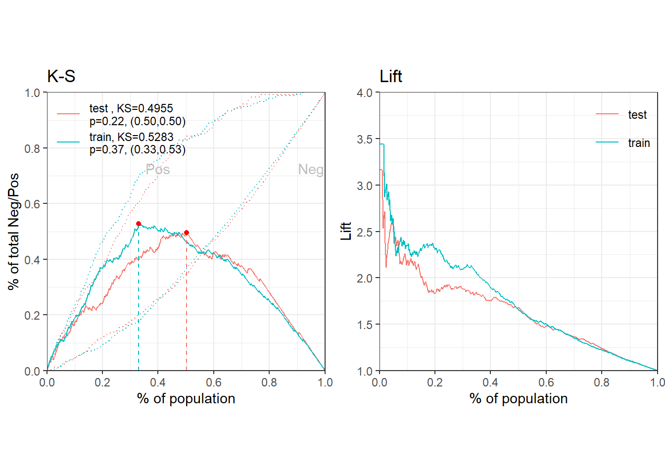
<- lapply (dt_woe_list, function (x) predict (m2, x, type = "response" ))<- perf_eva (pred = pred_list, label = label_list)
代码
$binomial_metric
$binomial_metric$train
         MSE      RMSE   LogLoss        R2        KS       AUC     Gini
       <num>     <num>     <num>     <num>     <num>     <num>    <num>
1: 0.1520812 0.3899759 0.4624491 0.2618686 0.5282828 0.8180745 0.636149

$binomial_metric$test
         MSE      RMSE   LogLoss        R2        KS       AUC      Gini
       <num>     <num>     <num>     <num>     <num>     <num>     <num>
1: 0.1695588 0.4117751 0.4990282 0.2152473 0.4955128 0.7998878 0.5997756


$pic
TableGrob (1 x 2) "arrange": 2 grobs
  z     cells    name           grob
1 1 (1-1,1-1) arrange gtable[layout]
2 2 (1-1,2-2) arrange gtable[layout]
创建评分卡
基于逻辑回归结果创建评分卡
代码
<- scorecard (bins_adj, m2,points0 = 600 , odds0 = 1 / 19 ,pdo = 50 , basepoints_eq0 = FALSE
$basepoints
     variable    bin    woe points
       <char> <lgcl> <lgcl>  <num>
1: basepoints     NA     NA    456

$status.of.existing.checking.account
                              variable
                                <char>
1: status.of.existing.checking.account
2: status.of.existing.checking.account
3: status.of.existing.checking.account
                                                      bin count count_distr
                                                   <char> <int>       <num>
1:                         ... < 0 DM%,%0 <= ... < 200 DM   543       0.543
2: ... >= 200 DM / salary assignments for at least 1 year    63       0.063
3:                                    no checking account   394       0.394
     neg   pos   posprob        woe      bin_iv total_iv
   <int> <int>     <num>      <num>       <num>    <num>
1:   303   240 0.4419890  0.6142040 0.225500603 0.639372
2:    49    14 0.2222222 -0.4054651 0.009460853 0.639372
3:   348    46 0.1167513 -1.1762632 0.404410499 0.639372
                                                   breaks is_special_values
                                                   <char>            <lgcl>
1:                         ... < 0 DM%,%0 <= ... < 200 DM             FALSE
2: ... >= 200 DM / salary assignments for at least 1 year             FALSE
3:                                    no checking account             FALSE
   points
    <num>
1:    -33
2:     22
3:     62

$age.in.years
       variable       bin count count_distr   neg   pos   posprob        woe
         <char>    <char> <int>       <num> <int> <int>     <num>      <num>
1: age.in.years [-Inf,26)   190       0.190   110    80 0.4210526  0.5288441
2: age.in.years   [26,35)   358       0.358   246   112 0.3128492  0.0604652
3: age.in.years   [35,40)   153       0.153   123    30 0.1960784 -0.5636891
4: age.in.years [40, Inf)   299       0.299   221    78 0.2608696 -0.1941560
        bin_iv  total_iv breaks is_special_values points
         <num>     <num> <char>            <lgcl>  <num>
1: 0.057921024 0.1127421     26             FALSE    -37
2: 0.001324476 0.1127421     35             FALSE     -4
3: 0.042679319 0.1127421     40             FALSE     39
4: 0.010817264 0.1127421    Inf             FALSE     14

$other.installment.plans
                  variable           bin count count_distr   neg   pos
                    <char>        <char> <int>       <num> <int> <int>
1: other.installment.plans bank%,%stores   186       0.186   110    76
2: other.installment.plans          none   814       0.814   590   224
     posprob        woe     bin_iv   total_iv        breaks is_special_values
       <num>      <num>      <num>      <num>        <char>            <lgcl>
1: 0.4086022  0.4775508 0.04593584 0.05759207 bank%,%stores             FALSE
2: 0.2751843 -0.1211786 0.01165623 0.05759207          none             FALSE
   points
    <num>
1:    -28
2:      7

$housing
   variable      bin count count_distr   neg   pos   posprob        woe
     <char>   <char> <int>       <num> <int> <int>     <num>      <num>
1:  housing     rent   179       0.179   109    70 0.3910615  0.4044452
2:  housing      own   713       0.713   527   186 0.2608696 -0.1941560
3:  housing for free   108       0.108    64    44 0.4074074  0.4726044
       bin_iv   total_iv   breaks is_special_values points
        <num>      <num>   <char>            <lgcl>  <num>
1: 0.03139265 0.08329343     rent             FALSE    -23
2: 0.02579501 0.08329343      own             FALSE     11
3: 0.02610577 0.08329343 for free             FALSE    -27

$duration.in.month
            variable       bin count count_distr   neg   pos   posprob
              <char>    <char> <int>       <num> <int> <int>     <num>
1: duration.in.month  [-Inf,8)    87       0.087    78     9 0.1034483
2: duration.in.month    [8,16)   344       0.344   264    80 0.2325581
3: duration.in.month   [16,34)   399       0.399   270   129 0.3233083
4: duration.in.month   [34,44)   100       0.100    58    42 0.4200000
5: duration.in.month [44, Inf)    70       0.070    30    40 0.5714286
          woe      bin_iv  total_iv breaks is_special_values points
        <num>       <num>     <num> <char>            <lgcl>  <num>
1: -1.3121864 0.106849463 0.2826181      8             FALSE     77
2: -0.3466246 0.038293766 0.2826181     16             FALSE     20
3:  0.1086883 0.004813339 0.2826181     34             FALSE     -6
4:  0.5245245 0.029972827 0.2826181     44             FALSE    -31
5:  1.1349799 0.102688661 0.2826181    Inf             FALSE    -67

$credit.history
         variable
           <char>
1: credit.history
2: credit.history
3: credit.history
4: credit.history
                                                                                      bin
                                                                                   <char>
1: no credits taken/ all credits paid back duly%,%all credits at this bank paid back duly
2:                                               existing credits paid back duly till now
3:                                                        delay in paying off in the past
4:                            critical account/ other credits existing (not at this bank)
   count count_distr   neg   pos   posprob         woe       bin_iv  total_iv
   <int>       <num> <int> <int>     <num>       <num>        <num>     <num>
1:    89       0.089    36    53 0.5955056  1.23407084 0.1545526808 0.2918299
2:   530       0.530   361   169 0.3188679  0.08831862 0.0042056484 0.2918299
3:    88       0.088    60    28 0.3181818  0.08515781 0.0006488214 0.2918299
4:   293       0.293   243    50 0.1706485 -0.73374058 0.1324227042 0.2918299
                                                                                   breaks
                                                                                   <char>
1: no credits taken/ all credits paid back duly%,%all credits at this bank paid back duly
2:                                               existing credits paid back duly till now
3:                                                        delay in paying off in the past
4:                            critical account/ other credits existing (not at this bank)
   is_special_values points
              <lgcl>  <num>
1:             FALSE    -70
2:             FALSE     -5
3:             FALSE     -5
4:             FALSE     41

$purpose
   variable
     <char>
1:  purpose
2:  purpose
3:  purpose
                                                                                               bin
                                                                                            <char>
1:                                                                         retraining%,%car (used)
2:                                                                                radio/television
3: furniture/equipment%,%domestic appliances%,%business%,%repairs%,%car (new)%,%others%,%education
   count count_distr   neg   pos   posprob        woe     bin_iv  total_iv
   <int>       <num> <int> <int>     <num>      <num>      <num>     <num>
1:   112       0.112    94    18 0.1607143 -0.8056252 0.05984644 0.1529244
2:   280       0.280   218    62 0.2214286 -0.4100628 0.04295896 0.1529244
3:   608       0.608   388   220 0.3618421  0.2799201 0.05011902 0.1529244
                                                                                            breaks
                                                                                            <char>
1:                                                                         retraining%,%car (used)
2:                                                                                radio/television
3: furniture/equipment%,%domestic appliances%,%business%,%repairs%,%car (new)%,%others%,%education
   is_special_values points
              <lgcl>  <num>
1:             FALSE     51
2:             FALSE     26
3:             FALSE    -18

$credit.amount
        variable         bin count count_distr   neg   pos   posprob
          <char>      <char> <int>       <num> <int> <int>     <num>
1: credit.amount [-Inf,1400)   267       0.267   185    82 0.3071161
2: credit.amount [1400,1800)   105       0.105    87    18 0.1714286
3: credit.amount [1800,4000)   382       0.382   287    95 0.2486911
4: credit.amount [4000,9200)   196       0.196   120    76 0.3877551
5: credit.amount [9200, Inf)    50       0.050    21    29 0.5800000
           woe       bin_iv  total_iv breaks is_special_values points
         <num>        <num>     <num> <char>            <lgcl>  <num>
1:  0.03366128 0.0003045545 0.1812204   1400             FALSE     -2
2: -0.72823850 0.0468153322 0.1812204   1800             FALSE     34
3: -0.25830746 0.0241086966 0.1812204   4000             FALSE     12
4:  0.39053946 0.0319870413 0.1812204   9200             FALSE    -18
5:  1.17007125 0.0780047502 0.1812204    Inf             FALSE    -54

$savings.account.and.bonds
                    variable
                      <char>
1: savings.account.and.bonds
2: savings.account.and.bonds
3: savings.account.and.bonds
                                                                   bin count
                                                                <char> <int>
1:                                                        ... < 100 DM   603
2:                                                 100 <= ... < 500 DM   103
3: 500 <= ... < 1000 DM%,%... >= 1000 DM%,%unknown/ no savings account   294
   count_distr   neg   pos   posprob        woe      bin_iv  total_iv
         <num> <int> <int>     <num>      <num>       <num>     <num>
1:       0.603   386   217 0.3598673  0.2713578 0.046647706 0.1909739
2:       0.103    69    34 0.3300971  0.1395519 0.002060052 0.1909739
3:       0.294   245    49 0.1666667 -0.7621401 0.142266143 0.1909739
                                                                breaks
                                                                <char>
1:                                                        ... < 100 DM
2:                                                 100 <= ... < 500 DM
3: 500 <= ... < 1000 DM%,%... >= 1000 DM%,%unknown/ no savings account
   is_special_values points
              <lgcl>  <num>
1:             FALSE    -14
2:             FALSE     -7
3:             FALSE     40
代码
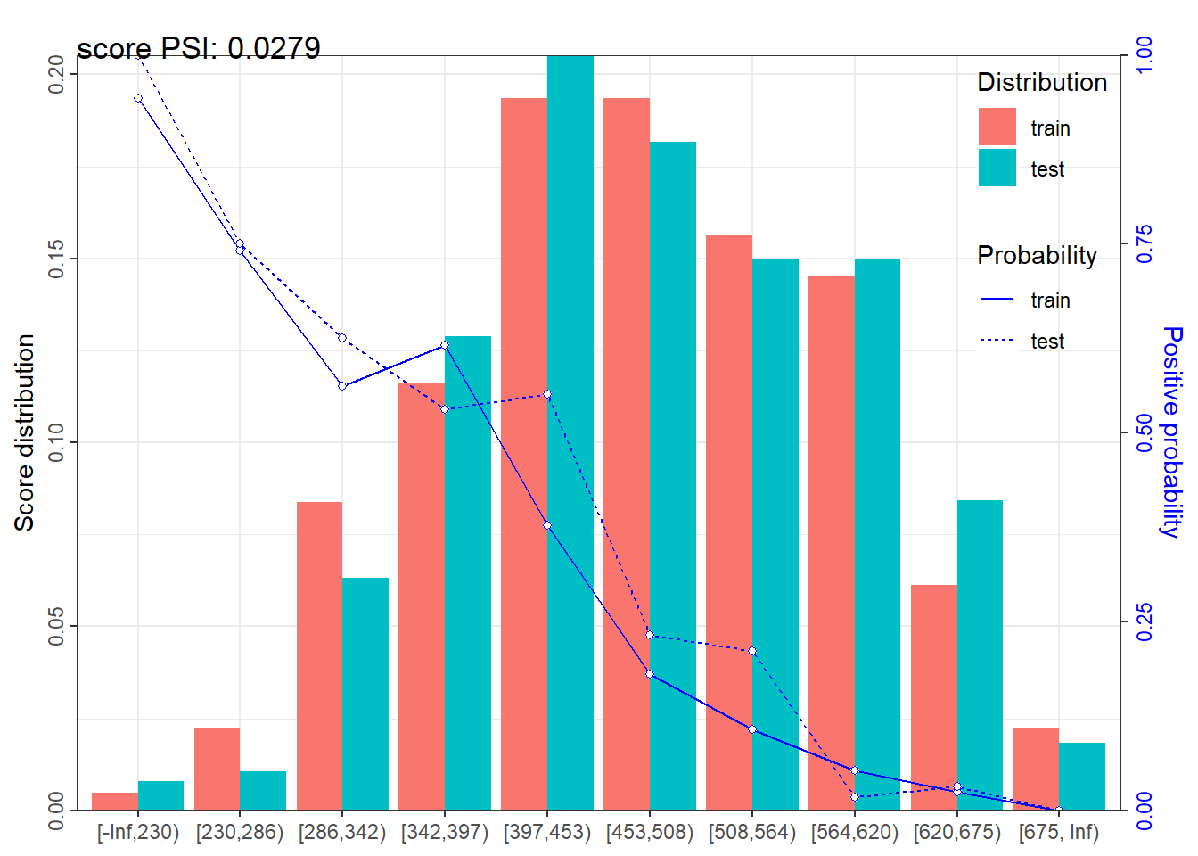
<- lapply (dt_list, function (x) scorecard_ply (x, card))perf_psi (score = score_list, label = label_list)
$psi
   variable    dataset        psi
     <char>     <char>      <num>
1:    score train_test 0.02792477